
In this article, we’ll take a deeper look at a fundamental classification of processors and its meaning in the audio production context. In particular, we’ll attempt to bridge the gap from theory to practical recommendations and guidelines, without relying on complex math or proofs.
One revolutionary advantage introduced by modern digital music production environments is practical linearity in recording, storage, amplification, filtering and playback. The following is meant to help the passionate audio engineer to better understand this environment, and optimally, push it to greater quality and efficiency.
This is a rather long read, without any audio. As an alternative, we suggest playing our latest compilation @ Spotify :)
Definition of system linearity
Linear systems show predictable behaviors that engineers can use to their advantage. Accordingly, nonlinear systems also show specific properties and limitations worth being aware of. The general definition of system linearity is:
A system is called linear if it has two mathematical properties: homogeneity and additivity. If you can show that a system has both properties, then you have proven that the system is linear. Likewise, if you can show that a system doesn’t have one or both properties, you have proven that it isn’t linear.The Scientist and Engineer’s Guide to Digital Signal Processing By Steven W. Smith, Ph.D.
Homogeneity requires the output level to be proportional to the input level. For example, if we amplify the input by 6dB, the output also increases by 6dB. If we half the input, the system also halves its output. From a practical point of view, it means that a linear system is generally independent of level: The effect remains exactly the same for both small and large signals.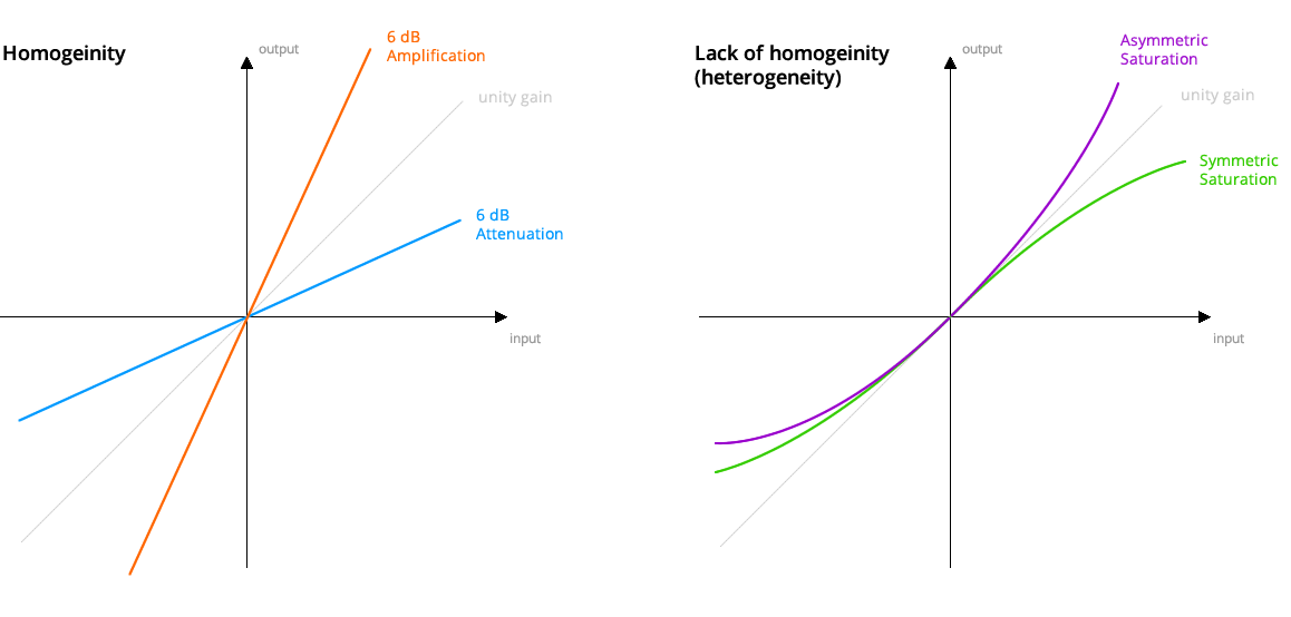
Additivity (also called “Superposition”) demands that the response caused by two or more sources is the sum of the responses that would have been caused by each source individually. This guarantees that no interaction appears between the different sources. Due to this property, linear processes can be separated, reordered and combined at a later point, while maintaining exactly the same results.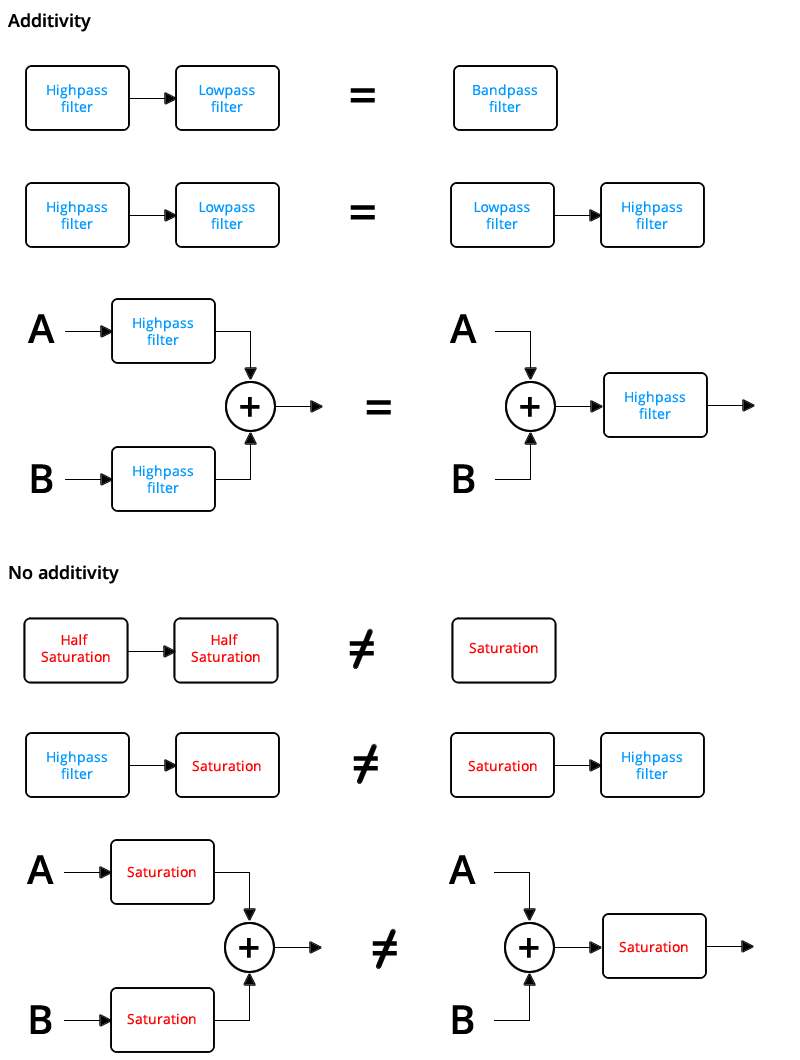
Probing for linearity
Let’s first understand how to verify for system linearity:
To get a better feeling for linearity, think about a technician trying to determine if an electronic device is linear. The technician would attach a sine wave generator to the input of the device, and an oscilloscope to the output. With a sine wave input, the technician would look to see if the output is also a sine wave. For example, the output cannot be clipped on the top or bottom, the top half cannot look different from the bottom half, there must be no distortion where the signal crosses zero, etc.
Next, the technician would vary the amplitude of the input and observe the effect on the output signal. If the system is linear, the amplitude of the output must track the amplitude of the input. Lastly, the technician would vary the input signal’s frequency, and verify that the output signal’s frequency changes accordingly. As the frequency is changed, there will likely be amplitude and phase changes seen in the output, but these are perfectly permissible in a linear system. At some frequencies, the output may even be zero, that is, a sinusoid with zero amplitude.
If the technician sees all these things, he will conclude that the system is linear. While this conclusion is not a rigorous mathematical proof, the level of confidence is justifiably high.The Scientist and Engineer’s Guide to Digital Signal Processing By Steven W. Smith, Ph.D.
In the modern audio processing context, we can simplify the experiment described above by focusing on effects that inevitably appear in systems that are not linear, i.e. systems that do not offer homogeneity and additivity (in pair).
All nonlinear systems, or more precisely, their underlying nonlinearities, produce partials that previously didn’t exist. Depending on the type of nonlinearity, these can be in harmonic relation to the signal, or not.
Today, most audio engineers have precise signal generators and FFT analyzers at their disposal. They allow us to replicate the above at great ease, and classify processors by running test signals through them while watching for partials appearing in the resulting spectrum.
We’ll use two signals. The first consists of a single sine wave at 630Hz: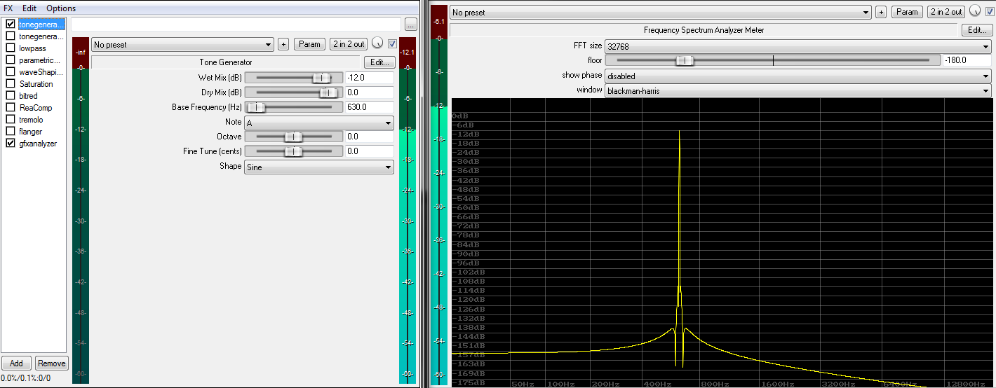 The second test signal is a sum of two sine waves, one running with 630Hz, the other with 880Hz. These chosen frequencies are arbitrary and have no deeper meaning. The important point is having at least two sines, as they offer a much better representation for real world audio signals than a single sine wave:
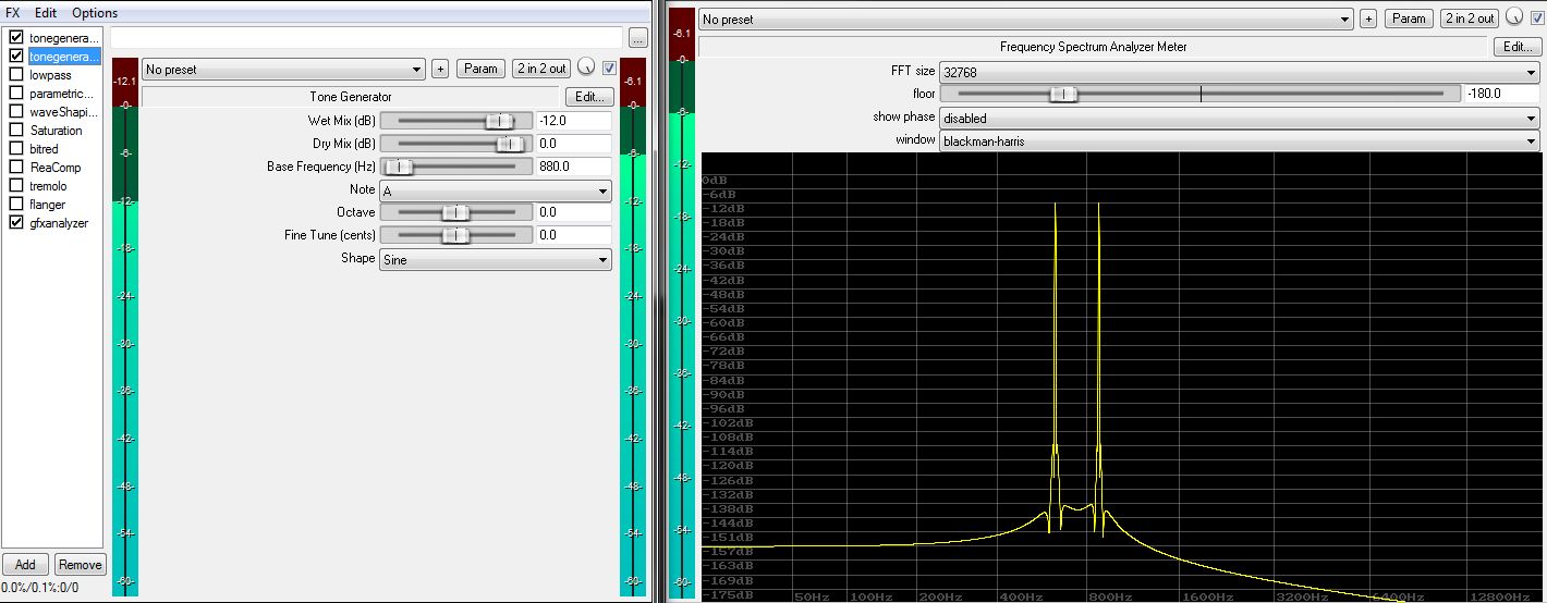
The test setup is made of a REAPER project. The project file can be downloaded at the bottom of this page.
A linear system cannot change the frequency of the original partial(s), and won’t produce new partials during the process. All a linear system can do is delay and/or amplify the input signal, or certain parts of it. If we spot a new partial, we can be certain to have a nonlinear system processing the signal.
Be aware that certain nonlinearities can have very complex mechanisms. Some have a deep relation to the signal history, while others show external dependencies and/or even very large linear regions. The fact that you can’t get a processor to generate any new partial doesn’t generally guarantee that the system is really linear. Though exceptions are unlikely in this field, most audio processors will quickly show their nature in this experiment, particularly with very high signal levels.
In fact, analogue circuit design differentiates between small signal models and large signal models. Small signal models can be fully described as networks of linear systems, a trick that greatly facilitates design and testing. However, if the signal grows too big (or too small), some components might be forced into their nonlinear regions. In this case, large signal models apply while small signal models start to yield questionable results. Large signals models usually turn out to be of far greater complexity of course.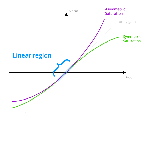 However, take this small vs large model classification with a grain of salt: Nonlinearities can very well be provoked by too low signal levels (e.g. hysteresis, quantization), or signal history, or interferences from external sources. They do not always depend on input level.
With the above, we can classify various systems according to their linearity.
Experiments
We’ll begin with a basic low pass filter:
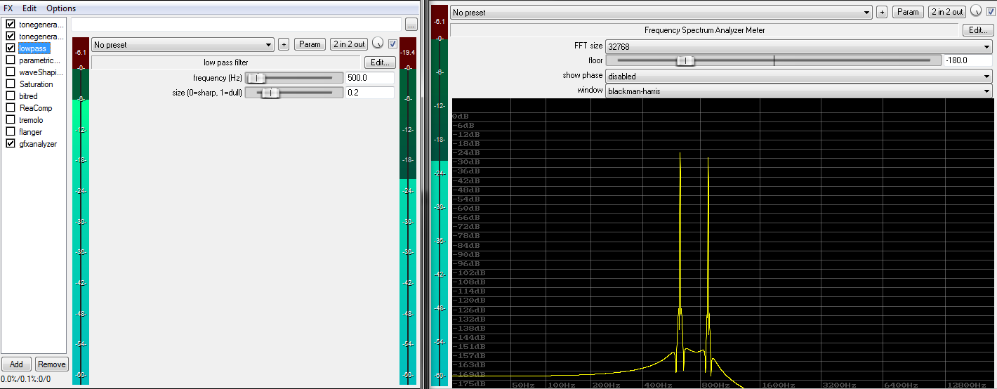 We can see the amplitudes of both the single sine wave and the sine wave pair being affected. You’ll notice that no partials appear, despite the fact that this filter is clearly acting on the two sine waves. We can assume that the system is linear.
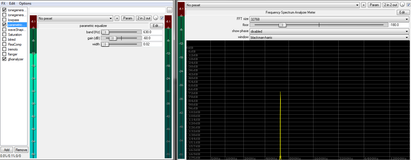
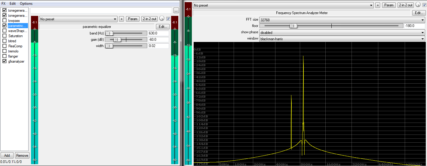
Here’s a narrow, and rather aggressive, peak filter. We can clearly see the 630Hz sine being attenuated, but without any partials appearing. This is also (very likely) a linear system:
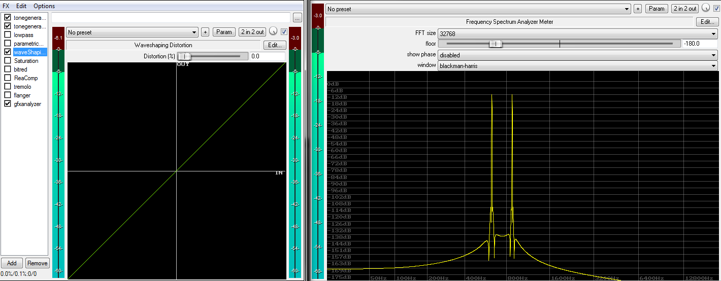
We’ll proceed with a simple waveshaper type saturator. Given a perfectly linear transfer function (waveshaper drive set to 0%), we obviously see the original input signal without any change. This is a linear system: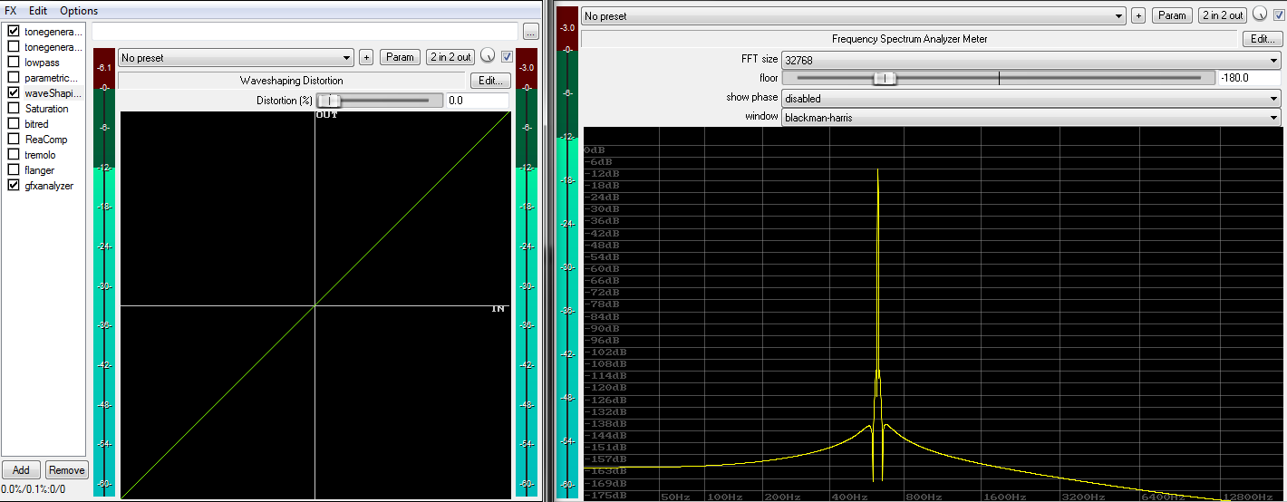
 We can now break the input/output linearity a little bit by increasing the waveshaper’s drive parameter. The effect is barely visible in the transfer curves, as they still look somewhat clean. However, the spectrum analyzer shows new partials appearing “out of the blue”. These in turn clearly reveal the presence of a nonlinearity:
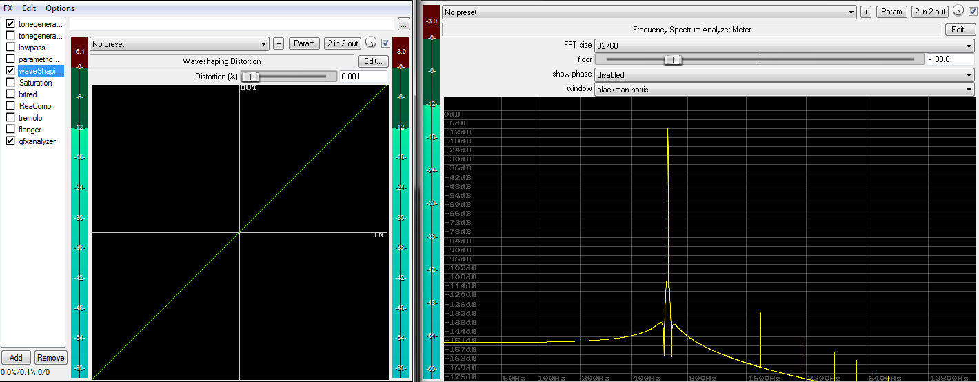
Some observations:
The low level of the generated partials relative to the original signal tells us that the nonlinearity is of relatively small extent.
The visually decaying amplitude of the resulting partials vs frequency tells us that the nonlinearity itself is likely continuous.
A high quantity of new partials appearing mean that we have a high order nonlinearity. Most nonlinearities are of high order once driven sufficiently. Meaning most of them have the potential to extend the original signal’s bandwidths by a near infinite amount. This makes it difficult to fulfill the laws of the sampling theorem (more about this later in the article).
The frequencies of the partials created in this example have an odd-numbered ratio to the original sine. Whole number ratios are called “harmonic”. This tells us the nonlinearity is symmetric with respect to signal polarity. Even a minute difference in symmetry would immediately generate even-numbered multiples of the original sine plus a DC component (the 0th harmonic), in addition to odd numbered multiples.
In comparison, our “sine wave pair” test-signal reveals more details:
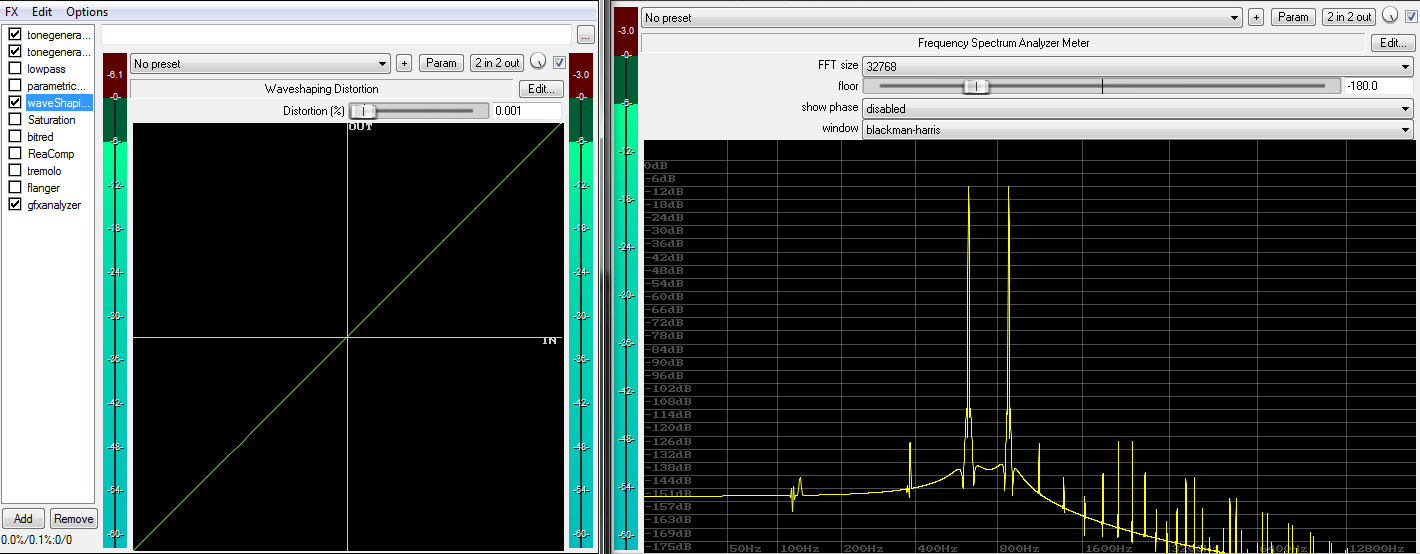 What can be seen here is the spectral effect of so called “inter-modulation distortion” (IMD). These numerous non-harmonic partials represent an often ignored “dark-side” of harmonic distortion. They have a sum/difference relation to the original sines that likely isn’t harmonic at all. Further, they are also likely to appear below the fundamental frequency.
From a technical point of view, IMD grows with two aspects:
1. The input signal’s bandwidth and spectral density (i.e. the width and density of the original signal’s partials).
2. The type and strength of nonlinearity.
As a rule of thumb, the narrower and simpler the input signal, the more harmonic the spectra returned by most nonlinearities. From a more practical view, IMD is the reason why an electric guitar can be distorted like crazy and still sound great. However, doing the same with a pop-song will likely not sound agreeable.
Let’s drive the saturator further: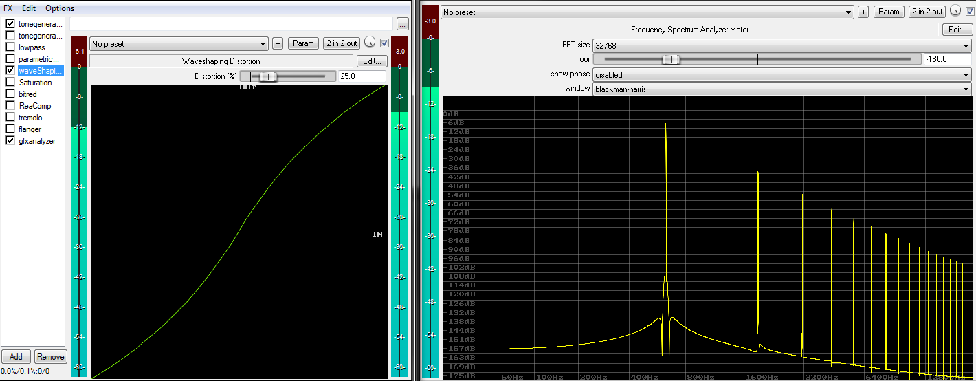
The harmonic nature now becomes very visible (input: single sine wave).
With two sine waves, the IMD becomes very obvious.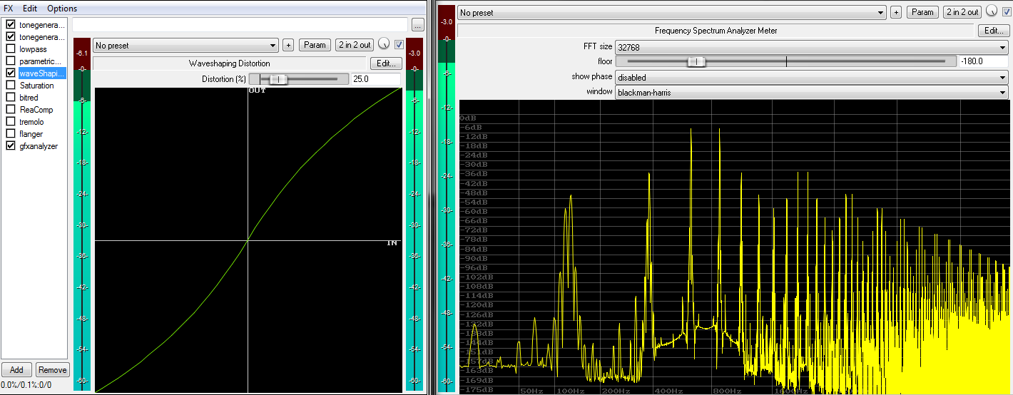
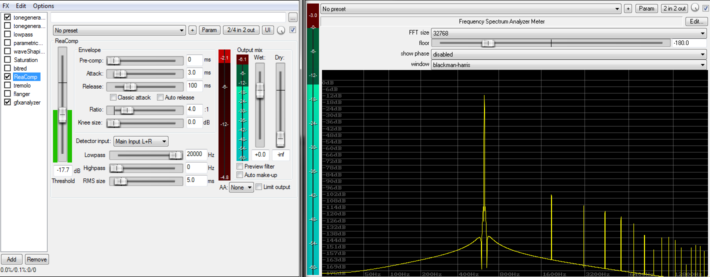
A dynamic range compressor doesn’t look much different. We can identify a rather smooth, continuous nonlinearity:
As before, the 2-sine wave picture reveals a significantly less harmonic “picture”, but distortion is still of very low amplitude. This system clearly is nonlinear of course.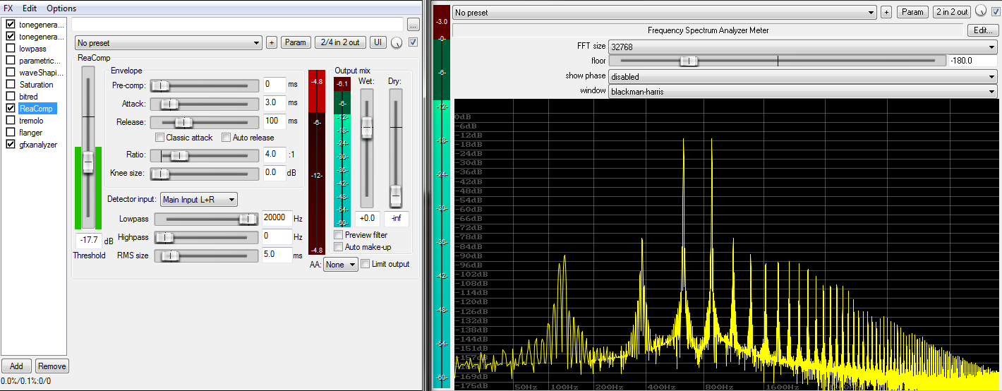
We’ll now take a look at modulation and special effects. Here’s a tremolo (an amplitude modulator):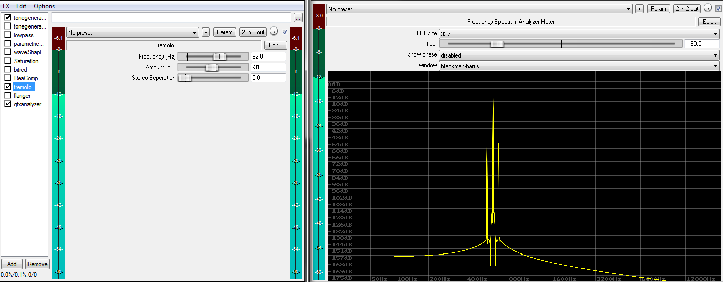
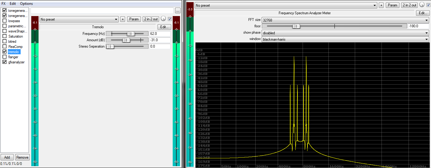
In the plots above, we clearly see new partials appearing. Modulation (and automation) turns any linear system into a nonlinear system. This also becomes obvious once we start modulating linear effects such as a delay, and mix it back into the original signal to create a flanger effect: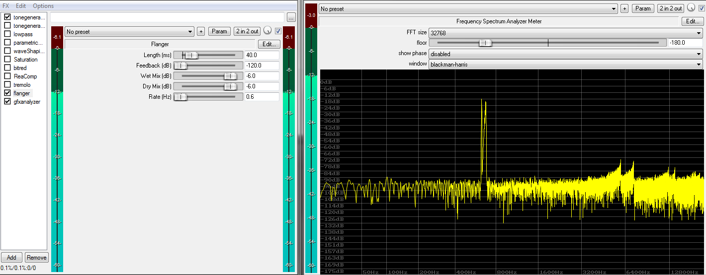
Noise
Note that all practical systems also involve a noise component. Noisy systems represent an edge case in our classification, they are arguably neither linear nor nonlinear. Hence engineers often separate the matter and talk about linear + noise or nonlinear + noise systems.
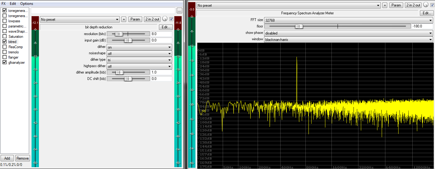
It’s worth mentioning a wonderful curiosity in this context. Let’s take a closer look at bit-depth reduction by using a so called “bit-crusher”. We’ll use it to truncate the word-length of our first test signal to 8 bit: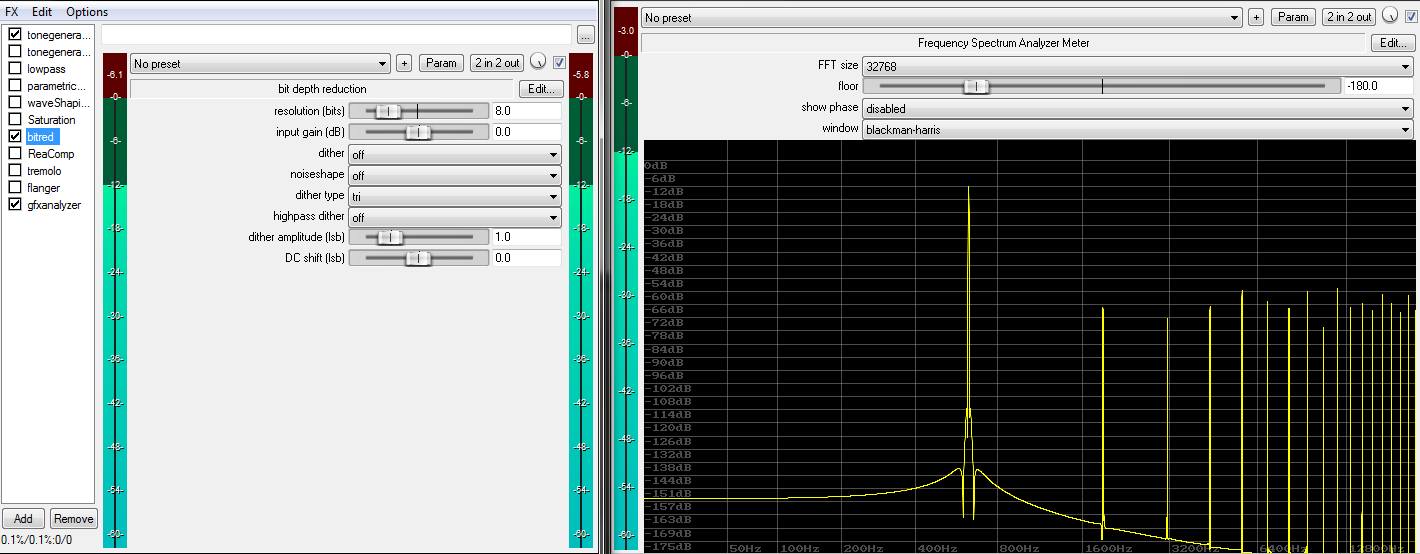
Again, additional partials, and thus a nonlinearity, are easily identified in the resulting spectrum. Note that contrary to the previous examples, partials do not attenuate with a growing frequency. Instead, the added partials exhibit a rather flat or even erratic spectrum. This is a clear sign for a discontinuity, which is a very sharp type of nonlinearity. This is what happens when a signal violently gets clipped, clamped, or truncated. Clippers produce similar spectra. After all, truncation is nothing more than low-level (i.e. zero-crossing) clipping.
Interestingly, injecting white noise of the right amplitude before truncation (i.e. “dithering” the signal prior to truncation) can literally turn this specific nonlinearity into a “linear process + noise”:
 The trick is that the signal removed by the truncation now purely consists of white noise rather than the original sine wave, so no partials can ever appear (noise is largely immune to nonlinearity). The truncation, in the dithered case, only happens in the noise floor of the signal. As long as the noise floor is greater than the signal to be removed by the truncation process, no quantization distortion or partials can appear.
A similar “wonder” happens in sample-rate conversion, where an adequately designed filter can turn an ugly decimation into a practically linear system (decimating means throwing samples away).
Some nonlinear systems, in certain situations, have the ability to create noise on their own, or at least something that looks very close to pure noise (i.e. pure randomness). Such belong to the class of chaotic systems, and find use in random number/noise generators.
Classification summary
| Linear | Nonlinear |
|---|---|
| Static delay Static amplification Static filtering Dithered truncation Bandlimited decimation (resampling) |
Saturation Dynamics processing Modulation Automation Pitch-shifting Raw truncation Raw decimation and many more processes |
Practical considerations
Homogeneity guarantees that linear systems don’t depend on gain staging strategies to operate properly. They are fully independent of the input signal level and/or history.
A nonlinear system on the other hand will likely saturate below or above at a certain level or after a certain signal history. An increase of 6 dB would only then maybe yield a result increased by 3 dB.
Many nonlinear systems have an almost linear region. Sensible gain staging then allows operating each processor within its mostly linear “sweet-spot”.
Additivity guarantees that the order of linear systems (e.g. amps, EQs, filters, delays), within a linear chain of other linear systems, can be changed arbitrarily without affecting the end result.
For example, it doesn’t matter whether the amp or EQ comes first. It also doesn’t matter whether a 30 Hz highpass filter sits on each track of a bus, or in a bus insert, as long there aren’t any nonlinearities in between. The CPU will greatly enjoy the simplification.
In contrast, a nonlinear system returns different outcomes in dependence of processing order. It makes a radical difference whether a saturator runs before or after any other processor. It also makes a difference if we’re to place one saturator per track, or inserting one into their bus. The “per track” case will likely sound clearer and more expressive (extreme creative destruction aside).
A linear system can only reduce the signal’s bandwidth, and cannot extend its bandwidth. It generally fulfills the sampling theorem, bandlimiting and aliasing is no issue. More precisely, a linear system is independent of samplerate.
Nonlinear systems on the other hand always increase the input signal’s bandwidth. They can potentially multiply the bandwidth up to infinity in no time, a fact that produces great trouble in the context of digital audio synthesis and processing. These systems have the inherent potential of breaking the Sampling Theorem, because new content ranging beyond the Nyquist frequency is likely to appear. If not handled properly, such content will directly produce alias images (also called Moiré patterns), a particularly nasty and irreversible form of distortion. Nonlinear systems, if not antialiased adequately, directly depend on sample-rate.
Inter-modulation-distortion (IMD) is a completely irreversible form of distortion. It appears as soon at least 2 sines meet a nonlinearity. The generated partials show no reasonable harmonic relation to the original signal. When problems appear, simplification and parallel processing structures often represent the only way out.
Nonlinear systems usually can’t be separated into smaller parts. For example, two weak saturators in series do not automatically generate less distortion than a single, “hotter” saturator! As a fact, they’d create less harmonic distortion, but more IMD. This is a reason why simplicity and minimalism is of such great value in music production.
An important aspect of linear systems is that they can be fully described by their impulse response. After all, system linearity means the signal can only become subject of fixed amplification, delay, and manipulations of the frequency and phase magnitude. This greatly helps designing, analyzing and verifying such systems at great speed, along with low cost and full predictability.
Nonlinear systems cannot be described by an impulse response, so they quickly become difficult to analyze and predict.
As a final remark, take note that no real world system is really fully linear. By strict standards, only theoretical constructs can really be fully linear. Nevertheless, well made analogue and most digital systems offer astonishingly wide linear regions. Digital audio processing in particular comes very close to the ideal of linearity, and this is a feature not to be underestimated!

